A Simulated Annealing FPGA Placer in Rust

This is about my journey in exploring FPGA placement algorithms as deeply as I can and sharing that with others in the simplest way I can. In the process, I also implemented a really simple toy FPGA placer in Rust. This topic is rarely explained in a clear way all in one place with references and a working implementation due to the topic being too niche yet highly fascinating. This is the motivation for me attempting to write as introductory of a post as I could make it, although still way longer than I hoped. Please note that almost every sentence in this post has additional context, detail, explanation, and complexity not addressed in this post for brevity, so I am most likely aware of many of the details you may point out that I have omitted, simplified, or modified.

I have recently been looking into FPGA placement and routing algorithms as part of my Ph.D. work to use deep learning to model and solve FPGA place-and-route problems directly. In the process, I also delved into the VPR codebase^[1] and more recent papers about electrostatic placement and routing tools, such as DreamPlace^[2] and the classic PathFinder negotiated congestion router paper^[3]. In the process, I was able to slowly pull apart the published research, trace back paper references, and build a mental understanding of the technical details and the history of research on the topic, an all-too-familiar process I have gone through during my Ph.D. It sure would be nice if there was something like this post that could have helped me get started.

I figured since I was already beginning to muck around in this topic area, I might as well have some fun on the side while learning Rust. It turned out to be a nice fit since the implementation of these algorithms is just as critical as the algorithm itself. Data structures and performance are critical since real place-and-route tools work on huge data structures such as netlist graphs and solve equally large and complex black-box optimization problems. Along the way, I don't want to make any silly, hard-to-debug errors as well, such as loose memory management (like you might in C/C++) or type errors (like you might in Python). Rust is advertised as a language that excels at these things by design, so I put it to the test. I recently wanted to learn Rust and needed to learn Rust. I wanted to learn Rust since we started to see if it would have any benefits in any of the research projects we are working on in my Ph.D. lab. Another student in our lab found great success breaking up parts of a project written in Python using Rust and the PyO3 library. Needing to learn Rust is a bit less cool since I need to know it for work.

In any case, I thought it would be fun to learn Rust by writing a toy simulated annealing FPGA placer.

If you already know what FPGA placement is and the different kinds of FPGA placement approaches and want to jump to the part about my implementation, you can skip to the section "My Simulated Annealing FPGA Placer", "Results and Visualizations", and "Source Code and Reproducibility".

What is an FPGA placer?

FPGA placement^[4] is very direct to formulate once you can be patient and build a simplified version of the problem.

I have a netlist graph that represents a circuit where the nodes are different circuit elements and the edges are wires. I also have an FPGA layout which is a 2D grid of spots where I can put a node. Each spot can only hold one circuit element and each spot can only hold one type of circuit element. In my toy prototype, there are only 4 types of circuit elements: CLBs, BRAM, DSP, and IO. Each node in the graph is one of these types and each spot on the FPGA layout can only fit one of these types. For example, some spots on the FPGA layout are only for IOs where I can place IO nodes from my graph on those spots.

Typically, we know that the FPGA layout will have more spots than needed to fit all the nodes in the graph. If this were not the case, we would not be able to fit all the nodes in the graph on the FPGA layout, and we could just stop there and tell the user that the FPGA layout is too small or their netlist is too big.

The goal of a placer is to map every node in your netlist to its own spot on the FPGA layout. If that were it, we could just list all the spots a node can go in and place it on the first available spot. We can then do this for all nodes until we are done.

In reality, after placement, we need to route the placed nodes together on the FPGA according to their edges in the netlist graph. A router will use the output solution generated by a placer to then route signals using the FPGA routing resources between placed nodes on the FPGA. If we randomly place two nodes far apart that are connected in the netlist graph, we will have to route a long wire between them. This is not good for several reasons, including timing and congestion. For this reason, we end up wanting to do this placement while minimizing the "distance" of placed nodes in the FPGA layout that are connected. This last minimizing objective is what makes placement a non-trivial problem.

How to solve FPGA placement?

Mix-Integer Linear Optimization

Given the set of nodes we need to place, the spots they can be placed in, constraints for 1-1 mapping, and constraints for mapping based on the node type, it is pretty cut-and-dry to formulate this problem as a mixed-integer optimization problem which has been studied for many years with solvers at the ready for us to use. The only thing is that we would have to formulate the wire length objective as a linear equation. Luckily, we can just use Manhattan or grid distance to do this (you can use absolute value in the objective of a linear optimization problem under certain cases with certain modeling transformations, including this case). The final objective is the sum of all grid distances between all pairs of placed nodes on the 2D FPGA layout, where the pairs map to all edges in the netlist graph.

This approach sounds nice, but in reality, is not scalable. Let's say we have an FPGA grid of $100\times 100=10,000$ CLB spots, and we have a $5,000$-node netlist of all CLBs to place. We would need an optimization variable that represents a node being placed in each spot. This would result in a $100\times 100\times 5000=50,000,000$ variable optimization problem. Real FPGAs and netlists are much larger than this. Therefore, the runtime of the solver is certainly not going to be great, and solvers will not be able to handle real-world sized problems. We could possibly make this more tractable by looking at non-linear formulation and relaxations of the problem that are not completely black-box to the solvers, but I have not gone down this rabbit hole yet.

Analytic and Electrostatic Placement

Analytic placement is a neat and practical solution to FPGA placement.

It originates from the idea of replacing both the objective function of wirelength and the constraints of non-overlapping placement using equivalent continuous formulations. It relaxes the fixed constraint nature of the FPGA problem to the continuous domain where locations and distances can be continuous values. By doing so, we can define the objective as a sum of distances of all the nodes using a distance function like Euclidean distance, or new functions like squared distance ($L^2$ space), and formulate the non-overlapping constraint as another objective function that models the density, "overlappingness", or "close-togetherness" of nodes (there are different ways to model this density component, but that is another rabbit hole to explore). This objective is referred to as the density penalty or density function.

To then solve placement, you optimize a new objective function which is equal to the wire length objective function plus some density function with a weight lambda. Lambda here controls the strength of the density function which you can control through the optimization to enforce legal placement or "spreading out" of nodes. Since this is a continuous problem, we can use a gradient-based optimization method to solve it, which has also been studied for a long time and has many solvers ready to use.

Up to this point, many in the field would broadly consider this approach to be an "analytical placer". However, we can take this one step further and make it an electrostatic placer. It models the entire system as an electrostatic system where the nodes are equivalent to positive charges, and the density function is equivalent to the electric potential. From here, you can then drive the particles to a location that minimizes the electric potential using the electric field itself as the gradient which "pushes" the nodes in the desired direction to spread out and settle into a final location.

With this approach, there are algorithmic components mixed in. An electrostatic placer can be used to get good enough continuous placement solutions but with some overlap or not fully aligned to the exact grid locations of the FPGA. We must then use a legalizer to "snap" the nodes to spots on the FPGA grid.

I won't go into much more detail, but there are many papers on both analytical and electrostatic placement^[5] and more are currently still being published on the topic. To the best of my understanding, electrostatic placement is the state of the art for at least ASIC placement and FPGA placement (I think, based on current academic publications and my educated guessing).

Simulated Annealing

Compared to the previously described approaches for placement, simulated annealing (SA)^[6] takes more of a top-down black-box approach to the problem. In fact, simulated annealing is a misnomer as you don't really need the "annealing" part to make it work for the FPGA placement problem.

In a traditional optimization context, simulated annealing models a problem as a system with a given current solution. Then we can jump to another solution and see if that solution is better. If the new solution is better, then we can pick that as our new current solution.

Now my use of the word "jump" is very loose. A simple thing to do is jump around randomly to other solutions and see if I can find anything better. However, the smarter idea and core of simulated annealing is to assign possible solutions to probabilities. Nearby solutions with small jumps are more likely to be picked than jumps to faraway solutions. At the beginning of the optimization, faraway solutions are defined as more probable, allowing us to jump around all over the place. But as time goes on, we can make faraway jumps less probable and make the jumps we take more likely to be close solutions. This is the "annealing" part of simulated annealing, whose name is derived from the physical process of annealing, repeatedly heating and cooling, metal.

In the context of FPGA placement, we can model the "current solution" as a valid placement solution of all nodes, and a "jump" as making a change to the current placement solution. This change can be picked from a set of actions such as swapping the location of two random nodes of the same type or moving a random node to another valid location. The objective is still the sum of the wirelengths of all the edges of nodes in the placed solution. We can then evaluate whether to accept or reject a move based on whether that move decreases the value of our objective function. In other words, a move creates a new solution with a lower objective function value than the current solution, we accept that move and keep going with new moves. If the move creates a new solution with a higher objective function value than the current solution, we reject that move, keep the current solution, and try another move.

The annealing part comes in when determining how far to move a node or how far away the two nodes we pick to swap are. At first, you might want to make moves or swaps over large distances or you might want to accept some percent of moves that don't improve the objective, but as time goes on, you want to make smaller moves and be less likely to select moves that don't improve the objective. This is the "annealing" part of simulated annealing in the context of FPGA placement. In this example, we have a linear annealing schedule with a higher "temperature" at the beginning and a lower "temperature" at the end. Temperature in this case is linked to the probability of accepting a move that does not improve the objective function or making moves that are further away.

However, as it turns out, you technically don't need this annealing part to make FPGA placement work. You can just randomly try different moves and accept or reject them based on whether they improve the objective function. This is what I did in my toy implementation of an FPGA placer just to keep it simple.

VTR/VPR is a popular academic FPGA EDA flow (with synthesis, packing, placement, and routing) that uses simulated annealing for its FPGA placer^[7]. They (the VPR authors) have many papers that talk about the details of their implementation, such as the actions they use and how they schedule the annealing part. They also have a more complex set of moves and ways to pick moves between nodes within a certain distance of each other. In more recent times, they have also explored using simple reinforcement learning techniques to learn how to pick which moves to make at each step.

My Simulated Annealing FPGA Placer

Specifications

My placer includes several components and simplifications to the problem:

• I consider only four types of nodes to place: CLB, BRAM, DSP, and IO.
• My netlist graph contains nodes and edges:
  • Each node is one of the four types.
  • Each edge represents a connection between two nodes, meaning they will need to be routed together later.
• My FPGA layout is a 2D grid of spots:
  • Each spot can hold only one node.
  • Each spot is designated for a specific type.
  • Each node can be placed only on a spot that matches its type.
  • An FPGA layout spot can also be of a special type, EMPTY, which means no node can be placed there.
• My simulated annealing solver is simple and does not include annealing:
  • There are three types of moves:
    • Swap two nodes of the same type.
    • Move a node to a random spot of the same type.
    • Move a node to a spot of the same type that is close to the centroid of all the nodes in the netlist graph.
  • The objective function is the sum of the wire lengths of all the edges in the netlist graph.
    • The distance between two nodes is the Manhattan distance between the spots they are placed on.
  • I accept a move if it improves the objective function.
  • For any step, I can try n_neighbors different random moves on the current solution and pick the best one.
  • A random initial placement must be provided to the placer to start with.

Netlist Graph

Initially, I wanted to model the netlist as a directed hypergraph. In the truest definition, circuits are really directed hypergraphs since one output can split off and go to multiple inputs. The wire that connects a single output to many inputs is the edge and encompasses all nodes.

However, I ended up not using hypergraphs in the final prototype for two reasons.

First, to do things properly, I needed to handle the extra complexity of nodes with ports and edges between nodes but only to certain ports. In digital circuits, a component such as a 4-input LUT will have 5 ports for wires to go "in to" and "out of" the component. You could model the component as a node, but then an edge actually connects to a port on the node rather than the entire node. Deciding how to model this can get a bit complex, and I did not want to think too hard about it.

Second, there were no directed hypergraph libraries or at least the existing hypergraph libraries were not well documented enough to find the directed versions or missing features I would expect a graph library to have. I looked into hypergraph^[8] and mhgl^[9], but as mentioned, there was no support for directed hypergraphs.

The reason I wanted to support directed hypergraphs is that I also wanted to possibly model signal direction in the future. For example, I want the output pin of a 4-input LUT to be the source and the downstream node input pins to be the sink in the hyperedge. I'm not sure this makes a difference for this toy placement problem, but I wanted to keep this in mind if I extended my prototype to also include a router. I wrote a very crude directed hypergraph module with a bad implementation, so I ended up not using it.

I settled on modeling the netlist as a directed graph of abstract nodes with the 4 node types I decided on in my specifications.

#[derive(Clone, Hash, PartialEq, Eq, Debug, Copy)]
pub enum MacroType {
    CLB,
    DSP,
    BRAM,
    IO,
}

#[derive(Clone, Hash, PartialEq, Eq, Debug, Copy)]
pub struct NetlistNode {
    pub id: u32,
    pub macro_type: MacroType,
}

#[derive(Debug, Clone)]
pub struct NetlistGraph {
    pub graph: petgraph::graph::DiGraph<NetlistNode, ()>,
}

I used the petagraph^[10] library for the graph itself. This is where I first encountered the Rust type system in a delightful way, via generics. I am able to pass a node type parameter to a Petagraph DiGraph struct, and it will now automatically enforce that type and code completion in my editor to that type when accessing nodes in the graph. I was so used to Python that it felt really cool to see it in action using Rust, even considering the fact that I use Mypy and type hints in Python.

I also implemented some simpler helper functions to obtain a summary of nodes.

impl NetlistGraph {
    fn new() -> NetlistGraph {
        NetlistGraph {
            graph: petgraph::graph::DiGraph::new(),
        }
    }

    pub fn all_nodes(&self) -> Vec<NetlistNode> {
        ...
    }

    pub fn count_summary(&self) -> FxHashMap<MacroType, u32> {
        ...
    }
}

In addition, I used rustworkx-core^[11] for random netlists graph generation to build to test the placer later on. The build_simple_netlist function builds an Erdős-Rényi random graph^[12]. You can parameterize this kind of random graph with the number of nodes and the probability of an edge between two nodes.

This won't model the properties of real netlist graphs but will be good enough to at least test the placer. In real netlists, you might have highly connected clusters of nodes that represent different hardware modules in your design. These modules are connected via buses of wires and composed together. However, even this high-level "module hierarchy" graph structure is modified and optimized into a new graph after synthesis and technology mapping.

I have omitted some of the non-essential parts of the code for this.

pub fn build_simple_netlist(n_nodes: u32, n_io: u32, n_bram: u32) -> NetlistGraph {
    let mut netlist = NetlistGraph {
        graph: gnp_random_graph(
            n_nodes as usize,
            0.02,
            None,
            || NetlistNode {
                id: rand::thread_rng().gen(),
                macro_type: MacroType::CLB,
            },
            || (),
        )
        .unwrap(),
    };

    // pick n_io random clbs and change their type to io
    // use choose_multiple to avoid duplicates
    ...

    // pick n_bram random clbs and change their type to bram
    // use choose_multiple to avoid duplicates
    ...

    // connect any disconnected nodes
    ...

    netlist
}

FPGA Layout

I modeled the FPGA layout as an FPGALayout type which contains a hashmap of FPGALayoutCoordinate types to FPGALayoutType. This way I can query the locations of nodes in the FPGA layout by their coordinates which would not be as eddicent as a giant 2D array or vector of vectors.

Additionally, I store the width and height of the FPGA layout that work with some helper functions to query any point in the layout with special logic to return FPGALayoutType::EMPTY if the coordinate is not in the hashmap or None if the coordinate is out of bounds.

There are also some helper functions to set different patterns of FPGALayoutType in the layout, such as config_corners, config_border, and config_repeat. These make things like setting all the outer edges of the FPGA layout to FPGALayoutType::IO or setting a repeating pattern of spaced FPGALayoutType::BRAM columns easy.

#[derive(Clone, Hash, PartialEq, Eq, Debug, Copy)]
pub enum MacroType {
    CLB,
    DSP,
    BRAM,
    IO,
}

#[derive(Clone, Hash, PartialEq, Eq, Debug)]
pub enum FPGALayoutType {
    MacroType(MacroType),
    EMPTY,
}

#[derive(Eq, Hash, PartialEq, Clone, Copy, Debug)]
pub struct FPGALayoutCoordinate {
    pub x: u32,
    pub y: u32,
}

impl FPGALayoutCoordinate {
    pub fn new(x: u32, y: u32) -> FPGALayoutCoordinate {
        FPGALayoutCoordinate { x, y }
    }
}

#[derive(Debug, Clone)]
pub struct FPGALayout {
    pub map: FxHashMap<FPGALayoutCoordinate, FPGALayoutType>,
    pub width: u32,
    pub height: u32,
}

impl FPGALayout {
    pub fn new(width: u32, height: u32) -> FPGALayout {
        FPGALayout {
            map: FxHashMap::default(),
            width,
            height,
        }
    }

    pub fn config_corners(&mut self, layout_type: FPGALayoutType) {
        ...
    }

    pub fn config_border(&mut self, layout_type: FPGALayoutType) {
        ...
    }

    pub fn config_repeat(
        &mut self,
        x: u32,
        y: u32,
        width: u32,
        height: u32,
        step_x: u32,
        step_y: u32,
        layout_type: FPGALayoutType,
    ) {
        ...
    }

    pub fn valid(&mut self) -> bool {
        ...
    }

    pub fn get(&self, coordinate: &FPGALayoutCoordinate) -> Option<FPGALayoutType> {
        if coordinate.x >= self.width || coordinate.y >= self.height {
            return None;
        }
        if !self.map.contains_key(coordinate) {
            return Some(FPGALayoutType::EMPTY);
        }
        self.map.get(coordinate).cloned()
    }

    pub fn count_summary(&self) -> FxHashMap<FPGALayoutType, u32> {
        ...
    }

    pub fn render_summary(&mut self) -> String {
        ...
    }

    pub fn render_ascii(&self) -> String {
        ...
    }
}

There is also a simple helper function to generate a simple test FPGA layout with, IOs on the outer edges (except for the corners), CLBs filled in the middle, and BRAMs in the middle every 10 columns.

pub fn build_simple_fpga_layout(width: u32, height: u32) -> FPGALayout {
    let mut layout = FPGALayout::new(width, height);

    layout.config_border(FPGALayoutType::MacroType(MacroType::IO));
    layout.config_corners(FPGALayoutType::EMPTY);
    layout.config_repeat(
        1,
        1,
        width - 2,
        height - 2,
        1,
        1,
        FPGALayoutType::MacroType(MacroType::CLB),
    );

    // evey 10 columns should be BRAM
    layout.config_repeat(
        10,
        1,
        width - 2,
        height - 2,
        10,
        1,
        FPGALayoutType::MacroType(MacroType::BRAM),
    );

    assert!(layout.valid());

    layout
}

The Placement Solution

I decided to model the solution as a PlacementSolution type that holds a reference to a netlist graph, a reference to an FPGA layout, and a hashmap of NetlistNode to FPGALayoutCoordinate. The actual core of the solution lies in the hashmap since that tells you where each node in the netlist is placed on the FPGA layout.

#[derive(Debug, Clone)]
pub struct PlacementSolution<'a> {
    pub layout: &'a FPGALayout,
    pub netlist: &'a NetlistGraph,
    pub solution_map: FxHashMap<NetlistNode, FPGALayoutCoordinate>,
}

Rather than showing the full implementation for this type, I will show selected parts of the implementation that are relevant to the placer.

First is the placement actions and action functions.

#[derive(Debug, Clone, Copy)]
pub enum PlacementAction {
    MOVE,
    SWAP,
    MOVE_DIRECTED,
}

The simplest action is to move a node to a random empty valid location.

pub fn action_move(&mut self) {
    let mut rng = rand::thread_rng();

    // Randomly select a node
    let node = match self.netlist.all_nodes().choose(&mut rng) {
        Some(n) => n.clone(),
        None => return,
    };

    // Get possible sites
    let possible_sites = self.get_possible_sites(node.macro_type);

    // Return if there are no possible sites
    if possible_sites.is_empty() {
        return;
    }

    // Randomly select a location
    let location = match possible_sites.choose(&mut rng) {
        Some(l) => l.clone(),
        None => return,
    };

    self.solution_map.insert(node, location);
}

The next action is to swap the locations of two nodes of the same type.

pub fn action_swap(&mut self) {
    let mut rng = rand::thread_rng();

    // Randomly select a node
    let node_a = match self.netlist.all_nodes().choose(&mut rng) {
        Some(n) => n.clone(),
        None => return,
    };

    // Filter nodes of the same type
    let nodes_same_type: Vec<NetlistNode> = self
        .netlist
        .all_nodes()
        .iter()
        .filter(|&&node| node.macro_type == node_a.macro_type)
        .cloned()
        .collect();

    // If no nodes of the same type, return
    if nodes_same_type.is_empty() {
        return;
    }

    // Randomly select another node (node_b) of the same type
    let node_b = match nodes_same_type.choose(&mut rng) {
        Some(n) => n.clone(),
        None => return,
    };

    // Clone the locations first to avoid borrowing issues
    let loc_a = self.solution_map.get(&node_a).cloned();
    let loc_b = self.solution_map.get(&node_b).cloned();

    // Perform the swap
    if let (Some(loc_a), Some(loc_b)) = (loc_a, loc_b) {
        self.solution_map.insert(node_a, loc_b);
        self.solution_map.insert(node_b, loc_a);
    }
}

The last action is to move a node to a location that is close to the centroid of all the nodes in the netlist graph. This is a bit more involved since I need to calculate the centroid and then find the closest valid location to the centroid. This is also an expensive move making the runtime of the placer slower. However, the move can help the placer converge to a better solution faster since moving nodes to the centroid will quickly lower the objective function value in big jumps, up to a certain point in the optimization process.

pub fn action_move_directed(&mut self) {
    let node_count = self.netlist.graph.node_count() as u32;

    if node_count == 0 {
        panic!("No nodes in netlist; cannot compute mean for MOVE_DIRECTED");
    }
    let x_mean = self
        .netlist
        .all_nodes()
        .iter()
        .map(|node| self.solution_map.get(node).unwrap().x)
        .sum::<u32>()
        / node_count;

    let y_mean = self
        .netlist
        .all_nodes()
        .iter()
        .map(|node| self.solution_map.get(node).unwrap().y)
        .sum::<u32>()
        / node_count;

    let mut rng = rand::thread_rng();

    // pick a random node
    let node: NetlistNode = self.netlist.all_nodes()[rng.gen_range(0..node_count as usize)];

    let valid_locations = self.get_possible_sites(node.macro_type);
    let valid_closest_location = valid_locations
        .iter()
        .min_by(|a, b| {
            let a_distance =
                (a.x as i32 - x_mean as i32).abs() + (a.y as i32 - y_mean as i32).abs();
            let b_distance =
                (b.x as i32 - x_mean as i32).abs() + (b.y as i32 - y_mean as i32).abs();
            a_distance.cmp(&b_distance)
        })
        .unwrap();

    // if the new location is futher away from the mean than the current location, return
    let current_location = self.solution_map.get(&node).unwrap();
    let current_distance = (current_location.x as i32 - x_mean as i32).abs()
        + (current_location.y as i32 - y_mean as i32).abs();
    let new_distance = (valid_closest_location.x as i32 - x_mean as i32).abs()
        + (valid_closest_location.y as i32 - y_mean as i32).abs();
    if new_distance > current_distance {
        return;
    }

    self.solution_map
        .insert(node, valid_closest_location.clone());
}

You can then dispatch these actions using another helper function.

pub fn action(&mut self, action: PlacementAction) {
    match action {
        PlacementAction::MOVE => self.action_move(),
        PlacementAction::SWAP => self.action_swap(),
        PlacementAction::MOVE_DIRECTED => self.action_move_directed(),
    }
}

Another key aspect of the placer is the objective function. I have mentioned things such as using distance functions for wire lengths and summing all edges in the netlist graph. I'm going to take a brief detour to talk more about objective functions for place-and-route^[13].

Traditionally, a "net" is what is usually referred to as a hyperedge in a hypergraph. For the abstract "connection" from an output pin of one node to all the input pins of other nodes, it can be called a net. Nets are motivated as an abstraction since you might physically draw one bending and branching rectilinear metal path in a chip to connect all the pins of a net, hence acting as one abstract "net".

The individual connections from one output pin to one input pin are what I consider an "edge". This maps directly to the edges in a graph when talking about abstract graphs in mathematics. I can turn a net into a set of edges by just enumerating all source-to-sink connections in the net hyperedge.

In general, a single "net" contains multiple "edges", and, technically, for placement, the directedness of these "nets" and "edges" don't matter (at least in the simple toy placement problem I have introduced).

Some objective functions are net-level objectives. One popular net-level objective is Half-Perimeter Wirelength (HPWL), where HPWL is equal to half the length of the perimeter of the encompassing rectangular bounding box of the net:

$$HPW{L}_e=\underset{i\in n}{max}(x_i)-\underset{i\in n}{min}(x_i)+\underset{i\in n}{max}(y_i)-\underset{i\in n}{min}(y_i)$$

where $n$ is a net, $i$ is a node in the net, and $x_i$ and $y_i$ are the x and y coordinates of node $i$. There are many proposed ways to relax the min and max functions to make this continuous, differentiable, and/or some version of convex as well as other related net-level objectives.

Assuming we just split all nets into edges, there are many net-level objectives, the simplest class of which are just distance functions in Euclidean space. Manhattan distance, aka "linear" wirelength model, is meant to model the optimal physical rectilinear routing of wires in a chip. This is formulated as $d_{ij}=|x_i-x_j|$ and the objective as $\sum _{e\in E}{d}_e=\sum _{e\in E}|x_i-x_j|+|y_i-y_j|$.

However, a more popular metric is the square distance, or the "quadratic" wirelength model. This is formulated as $d_{ij}=(x_i-x_j{)}^2$ and the objective as $\sum _{e\in E}{d}_e=\sum _{e\in E}(x_i-x_j{)}^2+(y_i-y_j{)}^2$.

In my toy placer, I use the linear wirelength model in my objective function since I am modeling everything as just edges and not nets. The naming of cost_bb is a bit of a misnomer since I am not computing anything related to the bounding box of the net. I am just summing the Manhattan distance of all edges in the netlist graph.

pub fn cost_bb(&self) -> f32 {
    let mut cost = 0.0;

    for edge in self.netlist.graph.edge_references() {
        let source_idx = edge.source();
        let target_idx = edge.target();

        let source = self.netlist.graph.node_weight(source_idx).unwrap();
        let target = self.netlist.graph.node_weight(target_idx).unwrap();

        let source_location = self.solution_map.get(source).unwrap();
        let target_location = self.solution_map.get(target).unwrap();

        let x_distance = (source_location.x as i32 - target_location.x as i32).abs();
        let y_distance = (source_location.y as i32 - target_location.y as i32).abs();

        let distance = x_distance + y_distance;
        cost += distance as f32;
    }

    cost
}

I also include two independent helper functions to generate initial placement solutions: a random placement approach, gen_random_placement, and a greedy placement approach, gen_greedy_placement. The greedy placement approach places a node in the first available spot in the top left direction of the FPGA layout. This allows an initial solution to have all nodes placed next to each other, but likely harder to optimize more compactly, compared to an initial solution where nodes are placed further apart on average, but easier to optimize.

There are additional functions in the PlacementSolution implementation, including a render_svg function to make all the visualizations in this post, along with a Renderer type with a render_to_video function in the implementation that calls imagemagick^[14] and ffmpeg^[15] to render a video and GIFs of the optimization process.

The Placer

The last component is the actual placer, which is surprisingly simple and compact to implement as a single function. This implementation explores multiple parallel moves at each step and picks the best move taken at that step. I also use rayon's^[16] par_iter feature to parallelize the exploration of moves at each step. This is a simple way to speed up the optimization process but might require some tuning since there might be some overhead in parallelizing the exploration of moves.

Ideally, there is a non-trivial tradeoff between the number of total steps taken and the number of parallel actions explored at each step. More actions-per-step results in it being more likely to find a better move at that single step, but more steps in total means more likely to reach a stable optimal solution, all with the tradeoff of total runtime. Maybe at different points in time during the optimization process, one would want to tune the number of parallel actions explored at each step. This is something I want to explore in the future and ties back directly to the "annealing" aspect of traditional simulated annealing. Changing the value of the number of actions explored at each step is what is referred to as building an annealing schedule, which also has parallels to picking learning rate schedules in deep learning.

pub struct PlacerOutput<'a> {
    pub initial_solution: PlacementSolution<'a>,
    pub final_solution: PlacementSolution<'a>,
    pub x_steps: Vec<u32>,
    pub y_cost: Vec<f32>,
    pub renderer: Option<Renderer>,
}

pub fn fast_sa_placer(
    initial_solution: PlacementSolution,
    n_steps: u32,
    n_neighbors: usize, // number of neighbors to explore at each step
    verbose: bool,
    render: bool,
) -> PlacerOutput {
    let mut renderer = Renderer::new();

    let mut current_solution = initial_solution.clone();

    let mut rng = rand::thread_rng();
    let actions: &[PlacementAction] = &[
        PlacementAction::Move,
        PlacementAction::Swap,
        PlacementAction::MoveDirected,
    ];

    let mut x_steps = Vec::new();
    let mut y_cost = Vec::new();

    for _i in 0..n_steps {
        x_steps.push(_i);
        y_cost.push(current_solution.cost_bb());
        if render {
            renderer.add_frame(current_solution.render_svg());
        }

        // randomly select actions
        let actions: Vec<_> = actions.choose_multiple(&mut rng, n_neighbors).collect();

        let new_solutions: Vec<_> = actions
            .into_par_iter()
            .map(|action| {
                let mut new_solution = current_solution.clone();
                new_solution.action(*action);
                new_solution
            })
            .collect();

        let best_solution = new_solutions
            .iter()
            .min_by(|sol1, sol2| {
                (sol1.cost_bb() - current_solution.cost_bb())
                    .partial_cmp(&(sol2.cost_bb() - current_solution.cost_bb()))
                    .unwrap()
            })
            .unwrap();

        let best_delta = best_solution.cost_bb() - current_solution.cost_bb();
        let mut delta = 0.0;
        if best_delta < 0.0 {
            current_solution = best_solution.clone();
            delta = best_delta;
        }

        if verbose {
            if _i % 10 == 0 {
                println!("Current Itteration: {:?}", _i);
                println!("Delta Cost: {:?}", delta);
                println!("Current Cost: {:?}", current_solution.cost_bb());
            }
        }
    }

    if render {
        renderer.add_frame(current_solution.render_svg());
    }

    PlacerOutput {
        initial_solution: initial_solution.clone(),
        final_solution: current_solution.clone(),
        x_steps: x_steps,
        y_cost: y_cost,
        renderer: if render { Some(renderer) } else { None },
    }
}

Results and Visualizations

To put it all together, I tested the placer as follows:

• A netlist with 300 nodes, 30 IOs, 100 BRAMs, and the rest as CLBs.
• An FPGA layout with a width of 64 and height of 64, with IOs on the outer edges, CLBs in the middle, and BRAMs every 10 columns.
• Each placer ran for 1000 steps.
• Run different trials of the placer with different values for n_neighbors = [1, 4, 8, 16, 32, 64, 128, 256]; each trial uses the same initial placement solution.

It works! The random initial placement and final placement solution using n_neighbors = 32 is shown below.

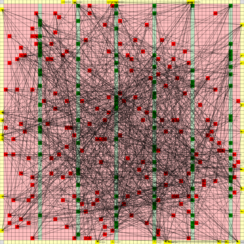
Random Initial Placement

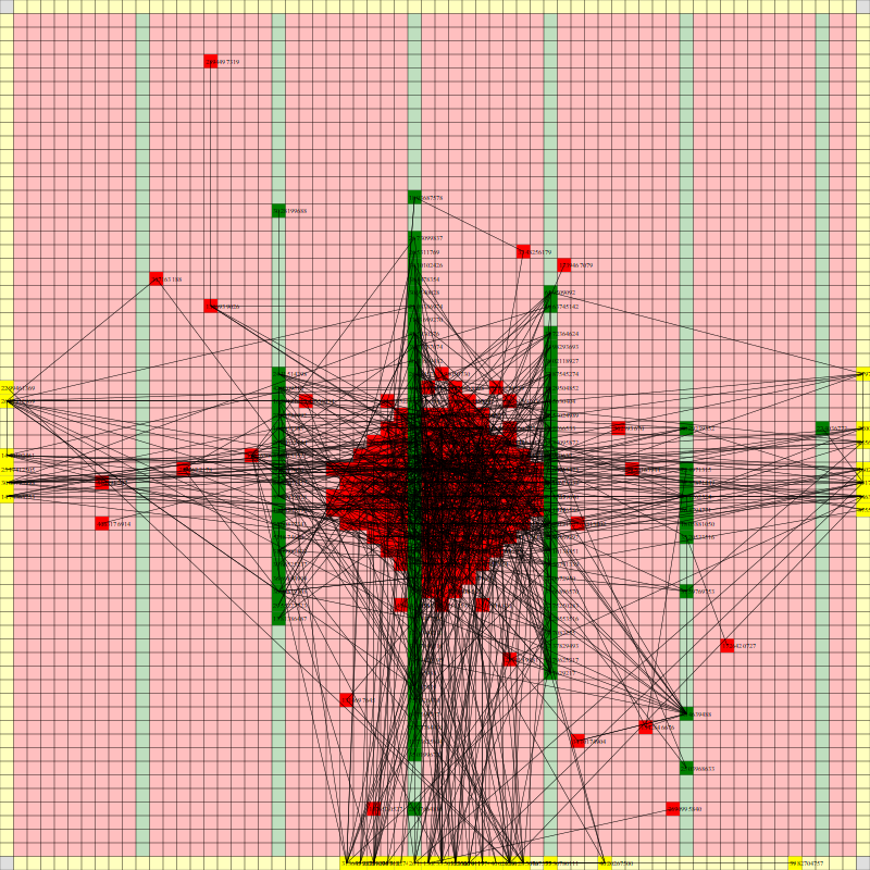
Final Placement Using n_neighbors = 32

Below is a video of the optimization process for this specific placement run, rendering every 20th step at 30 FPS.

The most notable aspect of this placer is that it tends to heavily rely on the directed move action to move nodes to the centroid of the netlist graph. I guess that starting from a random initial solution, these moves tend to be the most effective at lowering the objective function value. As time goes on and more nodes are placed in the center, this biases the directed moves to move nodes where all the nodes are in the middle. Random moves and swap moves, however, are still valuable for the placer to explore to optimize the placement of IOs since they are limited to the outer edges of the FPGA layout, and also BRAM since they have large jumps between the BRAM columns.

To also explore how the number of parallel neighbors explored at each step affects the optimization process. The results are shown below with the figure created using gnuplot^[17].

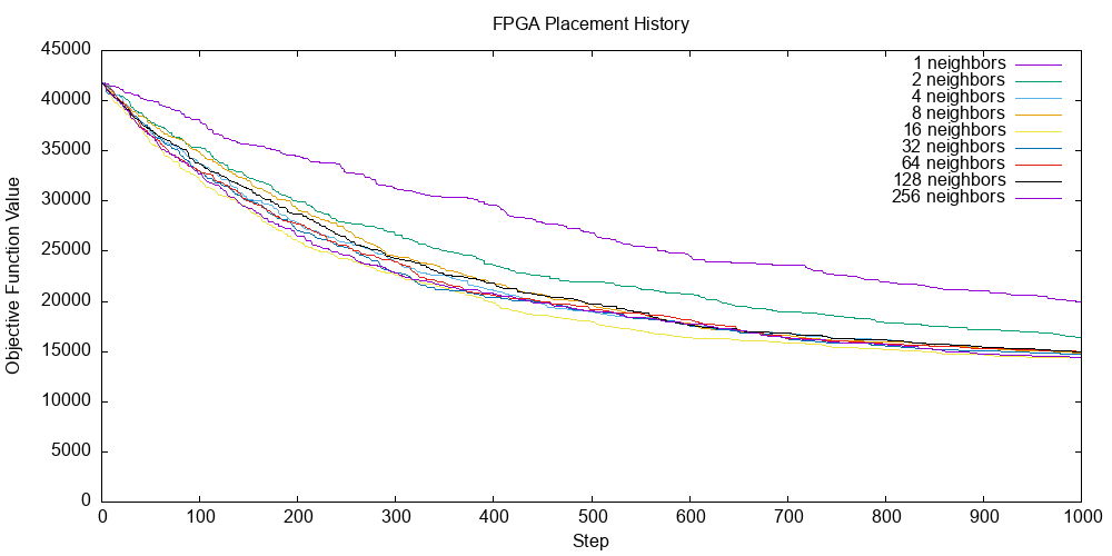
Exploring Placer Runs with Different Number of Parallel Neighbors

Intuitively, the placer run with the most number of neighbors explored in parallel is not the best at optimizing the placement objective function over the entire run. However, it seems that you want to search with 4 or more parallel neighbors as searching for 1 or 2 parallel neighbors is certainly not as effective.

It seems that there may be diminishing and then decreasing final objective values as you increase the number of parallel neighbors to search, but it is not yet clear to me what the optimal value is for parallel search at each step and what is going on here. This result is also very specific to the netlist and FPGA layout I used to test the placer. More diverse and comprehensive experiments are needed to draw more general conclusions.

Source Code and Reproducibility

You can find all the source code for this project here: https://github.com/stefanpie/sa-placer. This will let you dive into more details of the implementation that I omitted from this post as well as mess around with the code yourself and try different ideas. The generated data files (CSVs) and rendered visualizations (PNGs, MP4s, GIFs) are also in the repository.

Conclusion

There is not much more to say about the actual toy placer itself, but after this project, I do have some thoughts on EDA algorithms and EDA research that I think are important to say out loud.

It turned out that the ideas presented in journal and conference papers are much easier to understand once you can distill the core ideas and start from first principles. However, a lot of the published technical material on EDA is not very accessible or too surface level. I have found that textbooks and high-quality published course materials are good resources to break past the surface-level content. Furthermore, accessible and good quality (non-"research" quality) source code for advanced EDA algorithms are also hard to come by.

After using Rust for EDA, I have higher hopes and higher standards for better EDA software. I think there are huge gaps in performance in modern EDA tools and algorithms that, with some more investment in the software engineering and algorithms side of things, can be bridged. After using Rust, I think it is one of the best candidates for this kind of data structure and algorithm-heavy software with high standards for correctness and reliability.

Ideally, I would like to live in a world where it takes less than a minute to fully synthesize, place, and route a large modern FPGA design for a large modern FPGA device, something like a fast "prototype" flow that meets relaxed timing constraints. I think after this project, I can now see some glimmer of hope for this future.

Footnotes and References